8.1 Simple proportions

We often encounter problems where:

the number of items in the sample, denoted by $n$ , is fixed in advance;
there are two possible outcomes for each item (yes/no, success/failure, etc.);
each item has the same chance of producing a ‘success’, independently of all other items.

This leads to the Binomial model which describes the probabilities of the number of ‘successes’ out of the $n$ items, when the probability of success for a single item is $p$ .

If the number of ‘successes’ in the sample of size $n$ is $x$ then a natural estimate of $p$ is the sample proportion, $x / n$ . We write: $\hat{p} = x / n$

We need to quantify the uncertainty associated with estimating $p$ by $\hat{p}$ . As usual, the standard error does this for us.

The plot below uses simulation to show the variation in $\hat{p}$ when samples of size $n$ are repeatedly drawn from populations where the true proportion if $p$ . You might like to experiment with this code tp see the effectsd of changing n and p.

n <- 10
p <- 0.5
x <- rbinom(1000, n, p) 
hist(x / n, col = 'grey', xlim = c(0, 1), main = paste('n =', n, '  p =', p))
abline(v = p, col = 'red')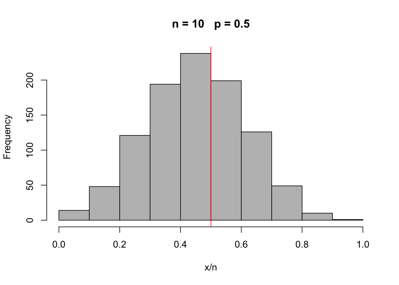

There are two simple points to note:

The sample proportion is subject to error but it is centred on the true proportion in the population.
The size of the error in the sample proportion decreases as the size of the sample increases.

In fact it is possible to show that the variance of $\hat{p}$ is $p (1 - p) / n$ . We can estimate the unknown $p$ in this expression to obtain the standard error $s . e . (\hat{p}) = \sqrt{\hat{p} (1 - \hat{p}) / n}$ As in other cases, we should find that most of the sample proportions lie within two standard errors of the true proportion. In this case we do not have an exact result for a confidence interval, as we do with the Normal model, but an approximate 95% confidence interval for $p$ is easily obtained as $\hat{p} \pm 2 s.e. (\hat{p})$ In a briefing note for journalists, the UK Parliament provides a helpful guide to opinion polls. (The document was prepared by Peter Kellner for the British Polling Council.) This refers to an accuracy of 3% in the main percentages reported in a poll based on 1000 respondents. Where does 3% come from?

When the sample size is 1000, the standard error of a proportion is $\sqrt{\hat{p} (1 - \hat{p}) / 1000}$ . The largest possible value of $\hat{p} (1 - \hat{p})$ is when $\hat{p} = 0.5$ , so the upper limit on the standard error is $\sqrt{0.5 \times 0.5 / 1000} = 0.16$ . Two standard errors is then 0.032, or around 3%.

This is a useful guide, but there are many other aspects of this to consider. We are often interested in comparing the proportions from different categories, such as support for the main parties in an election, and the uncertainty will be increased when two proportions are involved. In addition, there are all the usual issues about the extent to which the sampling is genuinely random or subject to bias of various kinds. Nonetheless, the ability of standard error to help in quantifying uncertainty is helpful.