3.2 Collating data from different sources
In the previous section, standard R functions were used to reorganise data. In principle, most things can be achieved by this route but the code can become complex to handle very detailed manipulations. As often happens, we can take advantage of the careful work of others by using packages which will help. The dplyr package is an excellent example. This provides powerful tools to manipulate data using high-level functions which take care of the details for us. Examples of these tools are described in this section.
This section also makes use of the readxl package to read Excel spreadsheets. Remember that packages need to be installed on your computer before they can be used, as was done for the rpanel package at the start of the book. The code below illustrates this for the two new packages we need, but it will be assumed for other package use later in the book. Installation needs to be done only once, with packages made available for a particular R session through the library function.
Example: Giving in the Church of England
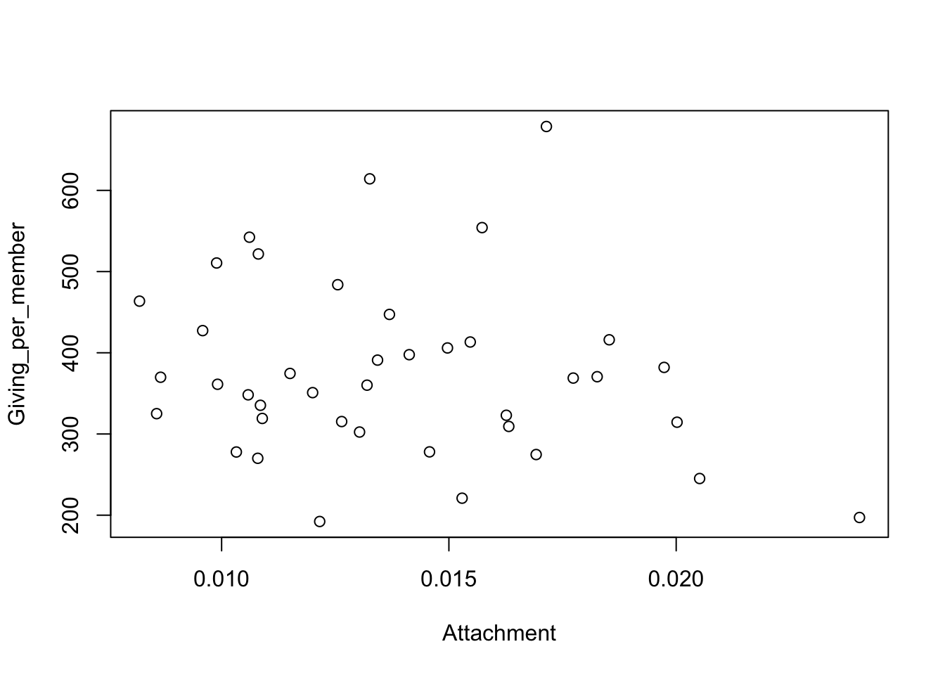
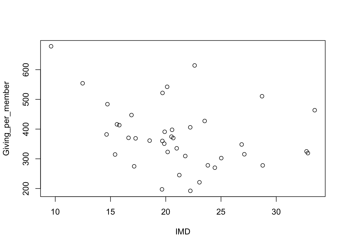
The Church of England is a large organisation whose 12,500 parishes, organised into 42 regions called dioceses, cover the whole of England. This gives a good context within which to explore patterns in charitable giving and Pickering (1985) examined this using data from the 1980’s. Prosperity (expressed in employment rate) and attachment (the proportion of the population associated with the church) were identified as important covariates associated with the variations in giving per church member across the country. Interestingly, giving per church member went down as attachment increased. Is this relationship still evident?The Data Services unit publishes a large amount of information about the composition and activity of the church so this provides an opportunity to examine whether these effects remain. However, the information required is spread across multiple files covering attendance, deprivation and giving. You may like to follow these links to look at the form and content of these spreadsheets.
The first task is to collate the information into a single dataset containing the appropriate data. We will focus on 2019 as this is pre-pandemic. The English Index of Multiple Deprivation (IMD) will be used as a measure of regional prosperity. It is appropriate to exclude Europe, the Channel Islands and the Isle of Man, for which some information is not available. These are also regions with unusual characteristics.
library(readxl)
library(dplyr)

path.attend <- rp.datalink('cofe_attendance_2019')
path.giving <- rp.datalink('cofe_giving_2019')
path.depriv <- rp.datalink('cofe_deprivation_2019')

d.elect <- read_excel(path.attend, sheet = 5, range = 'B4:I47')
d.elect <- select(d.elect, Diocese = 1, Elect = 3, Worship = 6)
The instructions above make use of the read_excel function to read an Excel spreadsheet. This includes helpful arguments to specify which sheet and which block of cells we would like to read from. The select function from the dplyr package then allows us to select out three columns of interest while simultaneously renaming them.
The last two operations can usefully be combined in the expression below. This uses the pipe operator. The results of the instruction preceding the %>% symbol are passed as the first argument of the instruction which follows. The select function expects a dataframe as its first argument. This allows multiple instructions to be combined in a natural order, without the need to use repeated <- assignments.
d.elect <- read_excel(path.attend, sheet = 5, range = 'B4:I47') %>%
   select(Diocese = 1, Elect = 3, Worship = 6)
We can apply this idea when reading the spreadsheets about attendance, giving and deprivation. The deprivation information is actually supplied at a finer level (parish) so the group_by and summarise functions allow us to aggregate to the level (diocese) which matches the information from the other spreadsheets.
d.attend <- read_excel(path.attend, sheet = 6, range = 'B4:D47') %>%
   select(Diocese = 1, Attend = 3)
d.giving <- read_excel(path.giving, sheet = 3, range = 'B8:BS49') %>%
   select(Diocese = 1, Giving = 19, Givers = 59)
d.depriv <- read_excel(path.depriv, sheet = 2, range = 'A1:AK12408') %>%
   select(Diocese = 11, population = 13, IMD = 37) %>%
   group_by(Diocese) %>%
   summarise(IMD = sum(IMD * population, na.rm = TRUE) /
                   sum(population, na.rm = TRUE),
             population = sum(population, na.rm = TRUE))
Before joining these different sets of information togethjer, it would be wise to check that there are no inconsistencies in the way the information has been coded. The anti_join function is very useful for this. Here is identifies some small differences in the names of the dioceses.
## # A tibble: 0 × 3
## # ℹ 3 variables: Diocese <chr>, Elect <dbl>, Worship <dbl>## # A tibble: 3 × 3
## Diocese Giving Givers
## <chr> <dbl> <dbl>
## 1 St.Albans 12579567 15283
## 2 St.Edmundsbury & Ipswich 4614832 8542
## 3 Sodor and Man 447514 623## # A tibble: 2 × 3
## Diocese IMD population
## <chr> <dbl> <dbl>
## 1 St.Albans 14.7 1927579.
## 2 St.Edmundsbury & Ipswich 17.1 679678.That can be fixed by using the mutate and recode functions.
d.attend <- mutate(d.attend, Diocese = recode(Diocese,
                   'St. Albans' = 'St.Albans',
                   'St. Edms & Ipswich' = 'St.Edmundsbury & Ipswich'))
d.elect  <- mutate(d.elect, Diocese = recode(Diocese,
                   'St. Albans' = 'St.Albans',
                   'St. Edms & Ipswich' = 'St.Edmundsbury & Ipswich'))
d.giving <- mutate(d.giving, Diocese = recode(Diocese,
                   'Sodor and Man' = 'Sodor & Man'))
Now we are in a position to join everything together using the full_join function, with a further adjustment to express attachment on a proportional scale and giving on a ‘per member’ scale.
cofe_2019 <- d.attend %>%
        full_join(d.elect,  by = 'Diocese') %>%
        full_join(d.depriv, by = 'Diocese') %>%
        full_join(d.giving, by = 'Diocese') %>%
        mutate(Attachment = Attend / population,
               Giving_per_member = Giving / Elect)
Now that the data have been collated into a single dataframe, we are ready to produce some plots which will address the question we began with. There is a lot of variation here. We will revisit this example in Chapter 9 when we discuss the topic of linear models.
plot(Giving_per_member ~ Attachment, data = cofe_2019)
plot(Giving_per_member ~ IMD, data = cofe_2019)

This example illustrates the power of the tools provided by the dplyr package. These manipulations could be performed through standard R functions but the code is likely to be much longer and more complex. A very useful resource is the summary sheet available from the RStudio menu Help > Cheat Sheets > Data Visualization with dplyr and on the web in html and pdf forms. This summarises the wide range of operations which dplyr supports.