12.2 Inference with simple flexible models

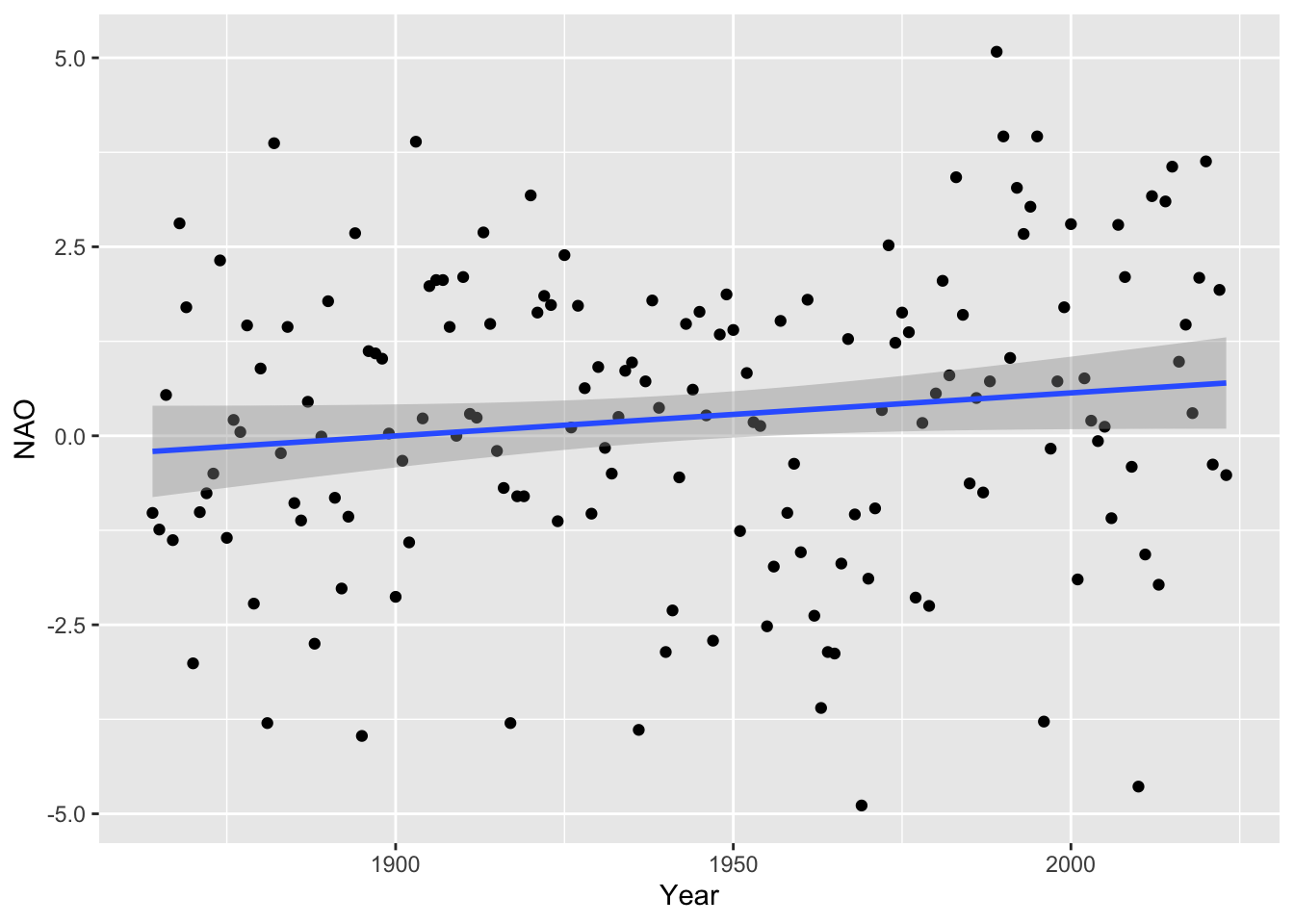
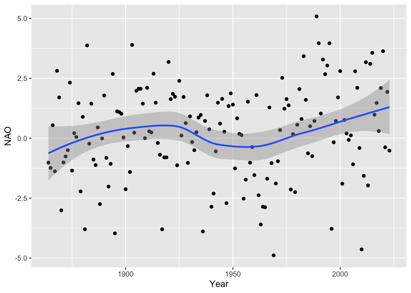
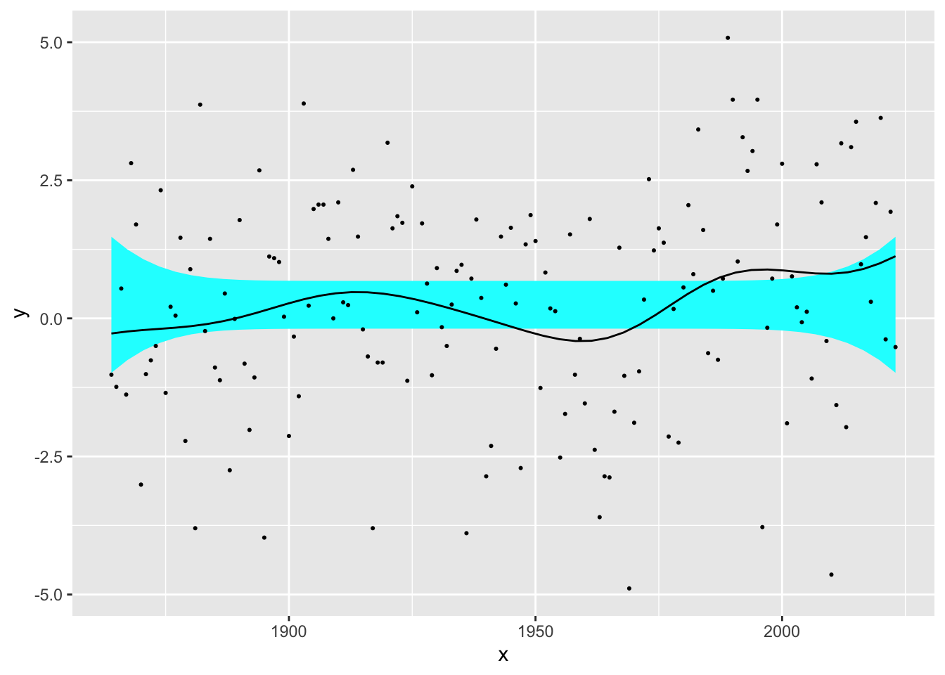
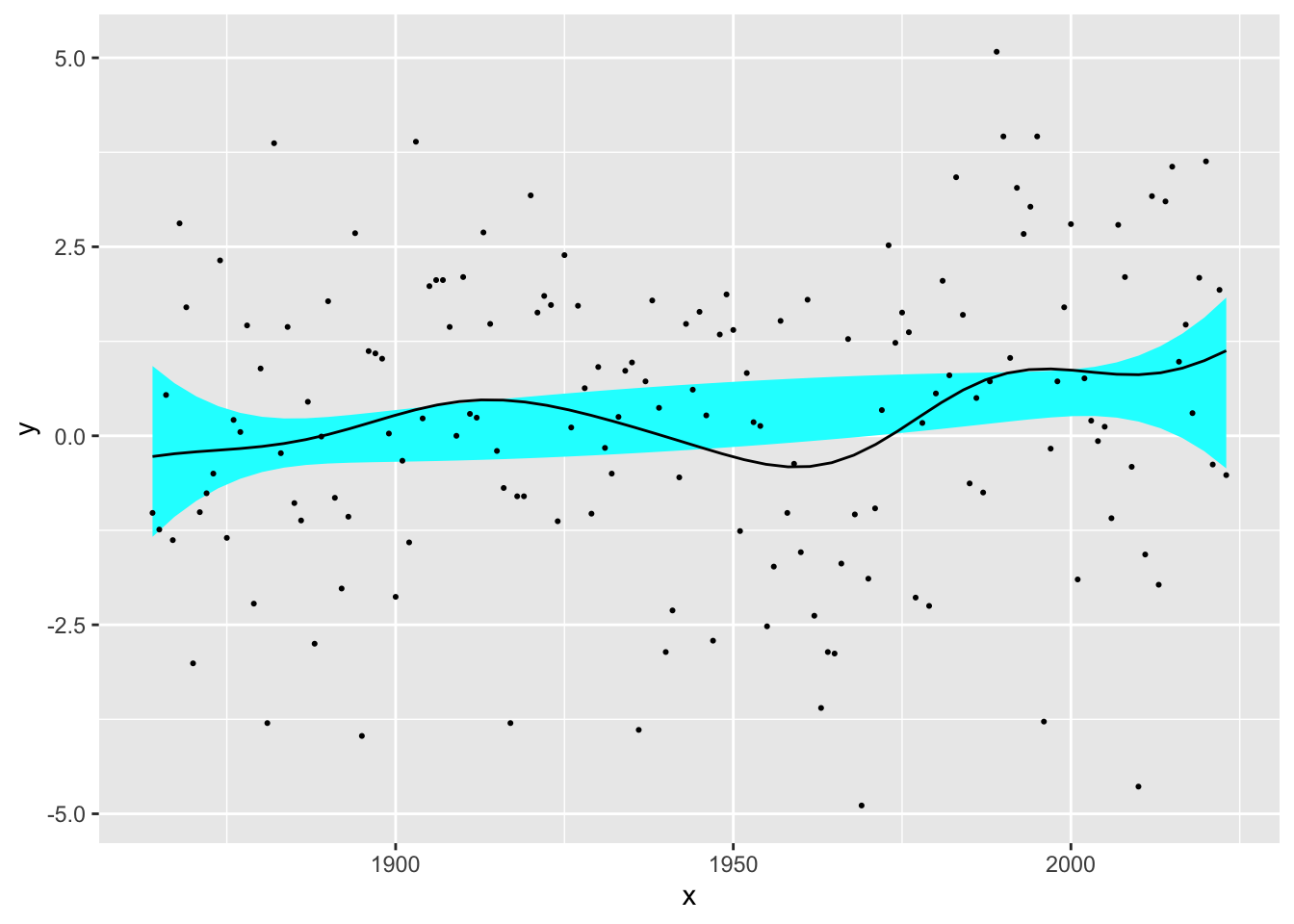
Historical data on Winter NAO data was discussed in Chapter on Trends and Patterns. If we fit a linear trend this is not significant. We can ask similar questions of the flexible regression: is there evidence of change of any kind?; is there evidence that this change is not linear? The flexible regression plots below display ‘reference bands’ which indicate where we expect the smooth curve to lie if indeed there is no trend at all, and in the second case if there is only linear trend. These graphical displays can be backed up by more formal methods which compare the sums-of-squares associated with the ‘no effect’, linear and smooth models. The calculation to produce p-values are a little more complex than in the standard case of linear models.

library(rpanel)
library(tidyverse)
library(sm)
path <- rp.datalink('NAO')
NAO  <- read.table(path, header = FALSE, skip = 1) %>%
   dplyr::select(Year = 1, NAO = 2)
ggplot(NAO, aes(Year, NAO)) + geom_point() + geom_smooth(method = 'lm')
summary(lm(NAO ~ Year, data = NAO))$coefficients
ggplot(NAO, aes(Year, NAO)) + geom_point() + geom_smooth()
sm.regression(NAO$Year, NAO$NAO, model = 'no effect')
sm.regression(NAO$Year, NAO$NAO, model = 'linear')

##                  Estimate  Std. Error   t value   Pr(>|t|)
## (Intercept) -10.812202830 6.469981059 -1.671134 0.09667481
## Year          0.005689807 0.003328096  1.709628 0.08929780
## Test of no effect model:  significance =  0.015 
## Test of linear model:  significance =  0.026