12.3 A simple additive model

Now that we have tools available to estimate smooth curves and surfaces, linear regression models can be extended to additive models as $$y_i={\beta }_0+s_1\left(x_{1i}\right)+\dots +s_p\left(x_{pi}\right)+{\epsilon }_i,i=1,\dots ,n.$$ The $m_i$ are functions whose shapes are unrestricted, apart from an assumption of smoothness and the constraint, for identifiability, that ${\sum }_i{s}_j\left(x_{ji}\right)=0$ for each $j$. As a consequence, we usually estimate ${\beta }_0$ by $\overline{y}$. This gives a very flexible set of modelling tools.

To see one approach to how these models can be fitted, consider the case of only two covariates, $$y_i={\beta }_0+s_1\left(x_{1i}\right)+s_2\left(x_{2i}\right)+{\epsilon }_i,i=1,\dots ,n.$$ A rearrangement of this as $y_i-{\beta }_0-s_2\left(x_{2i}\right)=s_1\left(x_{1i}\right)+{\epsilon }_i$ suggests that an estimate of component $m_1$ can then be obtained by smoothing the residuals of the data after fitting ${\hat{s}}_2$, $${\hat{m}}_1=S_1(y-\overline{y}-{\hat{s}}_2)$$ and that, similarly, subsequent estimates of $s_2$ can be obtained as $${\hat{m}}_2=S_2(y-\overline{y}-{\hat{s}}_1).$$ These smoothing operations are repeated until convergence. This is called the backfitting algorithm.

However, the regression and p-spline approaches described above allow models to be fitted directly. Each term $s_1,s_2,\dots$ can be represented by its own set of basis functions to create the usual linear model form $y=B\beta$, where $\beta$ now denotes a collections of several sets of coefficients, one for each term, and the columns of $B$ similarly cover the basis functions for all terms in the model. Combined with a set of penalty matrices and associated penalty parameters, the direct solution $\hat{\beta }=(B^{T}B+P{)}^{-1}{B}^{T}y$ still applies, where $P$ now denotes the sum of the individual penalty matrices weighted by their associated penalty parameters.

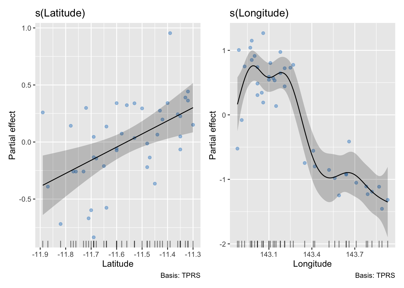
Here is an example of an additive model fitted to the trawl data. This uses the gam function in the mgcv package in R, which is a very powerful set of tools comprehensively described by Wood (2017). There are many options for how the model is fitted but here we will simply accept the defaults.

library(sm)
library(mgcv)
library(gratia)
ind         <- (trawl$Year==0 & trawl$Zone==1)
trawl.model <- gam(Score1 ~ s(Latitude) + s(Longitude), data = trawl, subset = ind)
draw(trawl.model, residuals = TRUE)

The non-linear effect of Longitude is apparent, as we saw in earlier examples. Here the model selection methods included in mgcv have led to a proposed linear relationship with Latitude.