4.4 Gaining an overview of datasets
Before starting serious analysis of any dataset, it is helpful to ‘screen’ the data by checking some basic features. For example, we might check the scales of measurement used, view the broad patterns of variation exhibited by individual variables, look out for unusual observations and so on. This is a kind of ‘sanity check’ which can highlight issues we may need to consider.
As an example, we will use data on herring gulls, as discussed in Section 1.1. (If you haven’t yet tried the data collection activity there, do go back and have a go.) Several measurements are available on each gull and the aim is to investigate whether these measurements can be used to classify birds as male or femal, as sex cannot easily be determined by inspection of the bird’s anatomy.
The dataset is hidden in the rpanel package, but we can retrieve it through the system.file command. Note the use of the stringsAsFactors argument of read.table which will ensure that any character variables are interpreted as factors. To improve the layout of results, a rather long variable name has also been slightly shortened.
path  <- system.file("extdata/gulls.txt", package = "rpanel")
gulls <- read.table(path, stringsAsFactors = TRUE)

library(tidyverse)
gulls <- rename(gulls, Head.Length = Head.and.Bill.Length)
How should we inspect this dataset? A first step might be to produce helpful summaries of each individual variable. The function summary is very useful as it adapts its output to the type of object it is passed, in this case a dataframe.
##      Weight        Wing.Length      Bill.Depth     Head.Length        Sex
##  Min.   : 705.0   Min.   :395.0   Min.   :15.70   Min.   :103.0   Female:210
##  1st Qu.: 860.0   1st Qu.:408.0   1st Qu.:17.50   1st Qu.:115.0   Male  :153
##  Median : 920.0   Median :417.0   Median :18.20   Median :119.0
##  Mean   : 948.1   Mean   :418.6   Mean   :18.41   Mean   :119.6
##  3rd Qu.:1042.5   3rd Qu.:429.0   3rd Qu.:19.30   3rd Qu.:125.0
##  Max.   :1250.0   Max.   :457.0   Max.   :22.50   Max.   :136.0
This provides a useful description of each variable, with quantiles for those on continuous scales and tabulations for factors. An alternative is the skim function from the skimr package which gives a little more information, provides some flexibility and fits neatly with the tidyverse. Here we improve the layout by omitting the complete_rate, as there are no missing data. The small histograms provide a neat graphical summary of the shape of the variability in each variable.
## ── Data Summary ────────────────────────
##                            Values
## Name                       gulls
## Number of rows             363
## Number of columns          5
## _______________________
## Column type frequency:
##   factor                   1
##   numeric                  4
## ________________________
## Group variables            None
##
## ── Variable type: factor ───────────────────────────────────────────────────────
##   skim_variable n_missing ordered n_unique top_counts
## 1 Sex                   0 FALSE          2 Fem: 210, Mal: 153
##
## ── Variable type: numeric ──────────────────────────────────────────────────────
##   skim_variable n_missing  mean     sd    p0   p25   p50    p75   p100 hist
## 1 Weight                0 948.  118.   705   860   920   1042.  1250   ▂▇▅▃▁
## 2 Wing.Length           0 419.   13.1  395   408   417    429    457   ▆▇▇▃▁
## 3 Bill.Depth            0  18.4   1.19  15.7  17.5  18.2   19.3   22.5 ▂▇▆▂▁
## 4 Head.Length           0 120.    6.50 103   115   119    125    136   ▁▇▅▆▁
Even at this stage, we should be guided by the aim of the analysis, which in this case is to assess the possibility of identifying the sex of a bird from its measurements. We could adapt the call to skim by inserting the dplyr function group_by(Sex) before it in a pipeline to create separate summaries for males and females. However, we are also interested in maximising the use of graphical exploration. Boxplots for each variable, separated by Sex, provide a good overall visual summary.
gulls %>%
   pivot_longer(cols = !Sex, names_to = "variable") %>%
   ggplot(aes(value, Sex)) + geom_boxplot() +
      facet_grid(. ~ variable, scales = 'free')
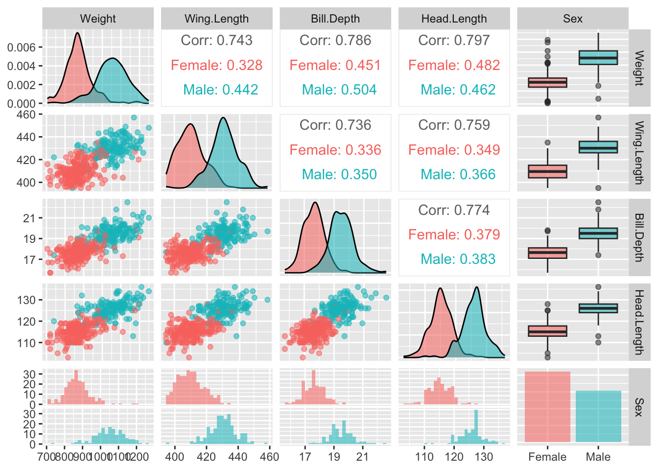
It is also helpful to gain an overview of the relationships between the variables. The ggpairs function in the GGally package can help with this. It provides a set of plots which incorporate a great deal of information in graphical form. As ever, there are various arguments we can use to control the details. Here colour is used to identify males and females. The stars argument is also used to suppress some information which is not relevant to us at this stage.
library(GGally)
ggpairs(gulls, aes(col = Sex, alpha = 0.7),
        upper = list(continuous = wrap(ggally_cor, stars = FALSE)))
The idea is to create a set of panels which plot each variable against every other one. The type of plot in each panel adapts to the nature of the variables involved. When both variables are on continuous scales, the relationship is summarised by correlation coefficients in the upper part of the matrix. The boxplots and histograms in the margins indicate that the separation of males and females on each individual variable is strong, which offers encouragement that effective classification may be possible.
These methods work well when the number of variables is small or modest. Large numbers of variables could be handled in appropriately chosen groups of variables, or by employing methods of dimension reduction, for example principal components.