8.3 Contingency tables

The data on smoking and lung cancer can also be treated as a simple example of a contingency table, which cross-classifies counts by two different factors. In fact, this was how the data were viewed in the original paper by Doll & Hill. The method of analysis we will explore can be implemented in contingency tables with any number of rows or columns.

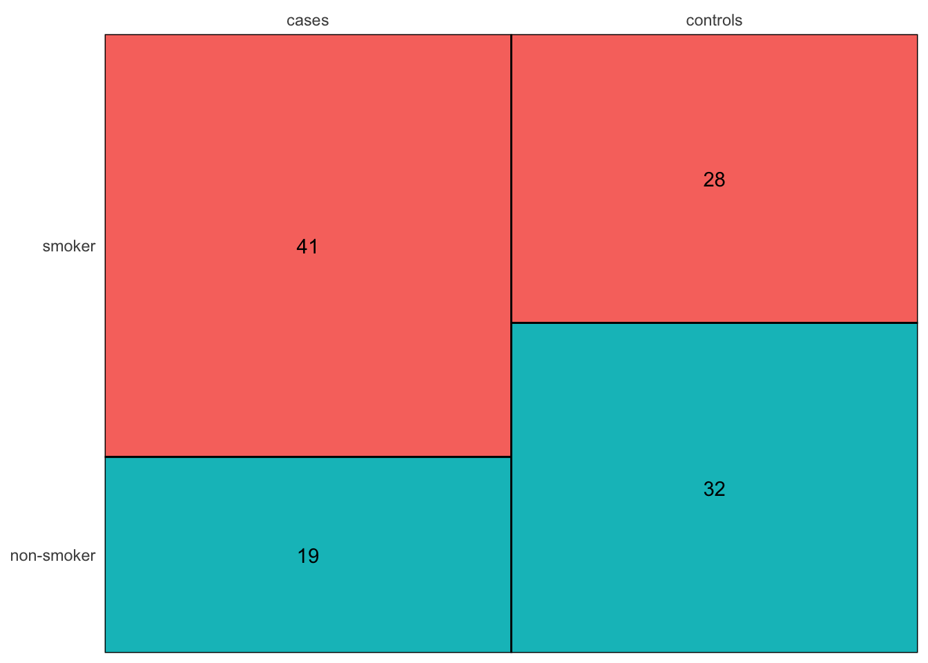
As ever, a helpful first step is to visualise the data, even when this consists of a very simple tabluation. The mosiacplot discussed earlier helps with this. The columns of the plot refer to the case and control groups. Here these are equal in size (60) but differences in in numbers would have been reflected in the width of the columns. This means that the height of each block now refers to proprtions of observations within each column.

x <- matrix(c(41, 19, 28, 32), ncol = 2,
            dimnames = list(c("smoker", "non-smoker"),
                            c("cases", "controls")))
rp.contingency(x)

If there is no association between smoking and lung cancer, then the proportions associated with each column will be identical. We can use this idea to calculate expected values, which describe the pattern we expect to see if the null hypothesis of no association is correct. Estimates of the common probabilities for each column are (69/120, 51/120) = (0.575, 0.425). The expected values by row are therefore obtained by multiplying the column totals by these probabilities. It so happens that the column totals are identical in this dataset, namely 60.

                            60 * 0.575, 60 * 0.575 = 34.5, 34.5
                            60 * 0.425, 60 * 0.425 = 25.5, 25.5

We can now compare this table of expected values ( $E_{i j}$ ) with the table of observed values ( $O_{i j}$ ) above. We do this through a quantity known as the chi-squared statistic, defined as $\sum_{i j} \frac{(O_{i j} - E_{i j})^{2}}{E_{i j}}$

where the subscripts $i$ and $j$ index the rows and columns. The chi-squared statistic for the current dataset is $5.76$ .

This value is meaningful only when we compare it to a reference distribution. The theory for this setting tells us that the relevant comparison is with a $χ^{2}$ distribution, which is plotted below. This distribution is indexed by a parameter known as the degrees of freedom. For contingency tables with $r$ rows and $c$ columns, the degrees of freedom should be set to $(r - 1) (c - 1)$ , which in the current case is $1$ .

library(rpanel)
rp.tables(panel = FALSE, distribution = "chi-squared", degf1 = 1, observed.value = 5.76)

The observed value of the test statistic, which is also shown in the plot, is much higher than values we expect to see from this reference distribution. The upper 5% point of the distribution is 3.84, which gives us a specific benchmark. We therefore have significant evidence that the proportions of smokers are different in the cases and controls. This formn of analysis has, unsurprisingly, confirmed the conclusions of the comparison of proportions in the previous section.

The chi-squared test can be easily implemented in R through the chisq.test function. By default this includes a correction for 2x2 tables in order to improve the accuracy of the reference distribution. However, the conclusion is unchanged.

chisq.test(x)

## 
##  Pearson's Chi-squared test with Yates' continuity correction
## 
## data:  x
## X-squared = 4.9105, df = 1, p-value = 0.02669